inferring cell-cell communication from scRNA-seq of ligand-receptor
2021/02/01 -- The reference LR datasets change to, core and extended, two parts. And change the tool name CellCall not CellWave.
The figure below shows a graphical representation of the CellCall workflow.

library(devtools)
devtools::install_github("ShellyCoder/cellcall")
If you encounter the following error -- ERROR: dependency * are not available for package 'cellcall', installing * package manually to install dependency is a good choice.
Specific functionalities of this package include (use data included in the package):
2.1 assessing how well ligands expressed by a sender cell interact with the receptor of receiver cell.
The colnames can't contain punctuation such as commas, periods, dashes, etc. Using underline to connect barcoder_celltype is recommended.
f.tmp <- system.file("extdata", "example_Data.Rdata", package="cellcall")
load(f.tmp)
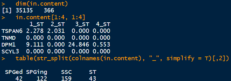
## gene expression stored in the variable in.content
dim(in.content)
in.content[1:4, 1:4]
table(str_split(colnames(in.content), "_", simplify = T)[,2])
What's important is the parameter as followed:
names.delim For the initial identity class for each cell, choose this delimiter from the cell's column name. E.g. If your cells are named as BARCODE_CELLTYPE, set this to "_" to separate the cell name into its component parts for picking the relevant field.
source the type of expression dataframe, eg "UMI", "fullLength", "TPM", or "CPM". If you don't want any transformation in the cellcall, using CPM data as input and set source = "CPM".
Org choose the species source of gene, eg "Homo sapiens", "Mus musculus". This parameter matters following ligand-receptor-tf resource.
  mt <- CreateNichConObject(data=in.content, min.feature = 3,
                            names.field = 2,
                            names.delim = "_",
                            source = "TPM", # fullLength, UMI, TPM
                            scale.factor = 10^6,
                            Org = "Homo sapiens",
                            project = "Microenvironment")
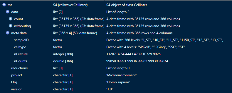
What's in the NichConObject ?
mt@data$count: raw data
mt@data$withoutlog: data proceeded by cellcall
mt@meta.data: metadata of the data, sampleID, celltype, etc
What's important is the parameter as followed:
names.delim For the initial identity class for each cell, choose this delimiter from the cell's column name. E.g. If your cells are named as BARCODE_CELLTYPE, set this to "_" to separate the cell name into its component parts for picking the relevant field.
mt <- TransCommuProfile(mt,
                          pValueCor = 0.05,
                          CorValue = 0.1,
                          topTargetCor=1,
                          p.adjust = 0.05,
                          use.type="median",
                          probs = 0.75,
                          method="weighted",
                          IS_core = TRUE,
                          Org = 'Homo sapiens')
What's new in the NichConObject ?
mt@data$expr_l_r: raw score
mt@data$expr_l_r_log2: log2(raw score+1)
mt@data$expr_l_r_log2_scale: do max,min transform to expr_l_r_log2
mt@data$gsea.list: result of TF-activation
set the color of each cell type
  cell_color <- data.frame(color=c('#e31a1c','#1f78b4',
                                   '#e78ac3','#ff7f00'), stringsAsFactors = FALSE)
  rownames(cell_color) <- c("SSC", "SPGing", "SPGed", "ST")
plot circle with cellcall object
ViewInterCircos(object = mt, font = 2, cellColor = cell_color, lrColor = c("#F16B6F", "#84B1ED"),
                  arr.type = "big.arrow",arr.length = 0.04,
                  trackhight1 = 0.05, slot="expr_l_r_log2_scale",linkcolor.from.sender = TRUE,
                  linkcolor = NULL, gap.degree = 2,order.vector=c('ST', "SSC", "SPGing", "SPGed"),
                  trackhight2 = 0.032, track.margin2 = c(0.01,0.12), DIY = FALSE)
plot circle with DIY dataframe of mt@data$expr_l_r_log2_scale

  ViewInterCircos(object = mt@data$expr_l_r_log2_scale, font = 2, cellColor = cell_color,
                  lrColor = c("#F16B6F", "#84B1ED"),
                  arr.type = "big.arrow",arr.length = 0.04,
                  trackhight1 = 0.05, slot="expr_l_r_log2_scale",linkcolor.from.sender = TRUE,
                  linkcolor = NULL, gap.degree = 2,order.vector=c('ST', "SSC", "SPGing", "SPGed"),
                  trackhight2 = 0.032, track.margin2 = c(0.01,0.12), DIY = T)

viewPheatmap(object = mt, slot="expr_l_r_log2_scale", show_rownames = T,show_colnames = T,
             treeheight_row=0, treeheight_col=10,
             cluster_rows = T,cluster_cols = F,fontsize = 12,angle_col = "45",
             main="score")

There are three types to show this triple relation.
Funtion LR2TF to measure the triple relation between specific cells.
  mt <- LR2TF(object = mt, sender_cell="ST", recevier_cell="SSC",
              slot="expr_l_r_log2_scale", org="Homo sapiens")
  head(mt@reductions$sankey)
First type, function LRT.Dimplot.
  if(!require(networkD3)){
  		BiocManager::install("networkD3")
  }

  sank <- LRT.Dimplot(mt, fontSize = 8, nodeWidth = 30, height = NULL, width = 1200, sinksRight=FALSE, DIY.color = FALSE)
  networkD3::saveNetwork(sank, "~/ST-SSC_full.html")
The first pillar is ligand,the second pillar is receptor,the last pillar is tf.
And the color of left and right flow is consistent with ligand and receptor respectively.

Second type, function sankey_graph with isGrandSon = FALSE.
library(magrittr)
library(dplyr)
tmp <- mt@reductions$sankey
tmp1 <- dplyr::filter(tmp, weight1>0) ## filter triple relation with weight1 (LR score)
tmp.df <- trans2tripleScore(tmp1)  ## transform weight1 and weight2 to one value (weight)
head(tmp.df)

## set the color of node in sankey graph
mycol.vector = c('#5d62b5','#29c3be','#f2726f','#62b58f','#bc95df', '#67cdf2', '#ffc533', '#5d62b5', '#29c3be')
elments.num <-  tmp.df %>% unlist %>% unique %>% length()
mycol.vector.list <- rep(mycol.vector, times=ceiling(elments.num/length(mycol.vector)))
sankey_graph(df = tmp.df, axes=1:3, mycol = mycol.vector.list[1:elments.num], nudge_x = NULL,
font.size = 4, boder.col="white", isGrandSon = F)
The first pillar is ligand,the second pillar is receptor,the last pillar is tf.
And the color of left and right flow is consistent with ligand and receptor respectively.

Third type, function sankey_graph with isGrandSon = TRUE.
library(magrittr)
library(dplyr)
tmp <- mt@reductions$sankey
tmp1 <- dplyr::filter(tmp, weight1>0)  ## filter triple relation with weight1 (LR score)
tmp.df <- trans2tripleScore(tmp1)  ## transform weight1 and weight2 to one value (weight)

## set the color of node in sankey graph
mycol.vector = c('#9e0142','#d53e4f','#f46d43','#fdae61','#fee08b','#e6f598','#abdda4','#66c2a5','#3288bd','#5e4fa2')
elments.num <-  length(unique(tmp.df$Ligand))
mycol.vector.list <- rep(mycol.vector, times=ceiling(elments.num/length(mycol.vector)))

sankey_graph(df = tmp.df, axes=1:3, mycol = mycol.vector.list[1:elments.num], isGrandSon = TRUE,
              nudge_x = nudge_x, font.size = 2, boder.col="white", set_alpha = 0.8)
The first pillar is ligand,the second pillar is receptor,the last pillar is tf.
And the color of left and right flow is consistent with one node (ligand or receptor).

getHyperPathway to perform enrichment, getForBubble to merge data for graph and plotBubble produce the bubble plot.
n <- mt@data$expr_l_r_log2_scale

pathway.hyper.list <- lapply(colnames(n), function(i){
    print(i)
    tmp <- getHyperPathway(data = n, object = mt, cella_cellb = i, Org="Homo sapiens")
    return(tmp)
})

myPub.df <- getForBubble(pathway.hyper.list, cella_cellb=colnames(n))
p <- plotBubble(myPub.df)

plot enrichment result of TF (filter or not).
## gsea object
egmt <- mt@data$gsea.list$SSC

## filter TF
egmt.df <- data.frame(egmt)
head(egmt.df[,1:6])
flag.index <- which(egmt.df$p.adjust < 0.05)

ridgeplot.DIY(x=egmt, fill="p.adjust", showCategory=flag.index, core_enrichment = T,
                orderBy = "NES", decreasing = FALSE)

  ssc.tf <- names(mt@data$gsea.list$SSC@geneSets)
  ssc.tf
Show all TF have result in the SSC.

  getGSEAplot(gsea.list=mt@data$gsea.list, geneSetID=c("CREBBP", "ESR1", "FOXO3"), myCelltype="SSC",
              fc.list=mt@data$fc.list,  selectedGeneID = mt@data$gsea.list$SSC@geneSets$CREBBP[1:10],
              mycol = NULL)

• Session info ------------------------------------------------------------------------------------------------
setting  value
version  R version 3.6.0 (2019-04-26)
os       Windows 10 x64
system   x86_64, mingw32
ui       RStudio
language en
• Packages ----------------------------------------------------------------------------------------------------
package         * version    date       lib source
AnnotationDbi     1.48.0     2019-10-29 [1] Bioconductor
assertthat        0.2.1      2019-03-21 [1] CRAN (R 3.6.3)
backports         1.1.7      2020-05-13 [1] CRAN (R 3.6.3)
Biobase           2.46.0     2019-10-29 [1] Bioconductor
BiocGenerics      0.32.0     2019-10-29 [1] Bioconductor
BiocManager       1.30.10    2019-11-16 [1] CRAN (R 3.6.3)
BiocParallel      1.20.1     2019-12-21 [1] Bioconductor
bit               1.1-15.2   2020-02-10 [1] CRAN (R 3.6.2)
bit64             0.9-7      2017-05-08 [1] CRAN (R 3.6.2)
blob              1.2.1      2020-01-20 [1] CRAN (R 3.6.3)
callr             3.4.3      2020-03-28 [1] CRAN (R 3.6.3)
cellcall        * 0.0.0.9000 2021-02-01 [1] local
circlize          0.4.10     2020-06-15 [1] CRAN (R 3.6.3)
cli               2.0.2      2020-02-28 [1] CRAN (R 3.6.3)
clue              0.3-57     2019-02-25 [1] CRAN (R 3.6.3)
cluster           2.0.8      2019-04-05 [1] CRAN (R 3.6.0)
clusterProfiler   3.14.3     2020-01-08 [1] Bioconductor
colorspace        1.4-1      2019-03-18 [1] CRAN (R 3.6.3)
ComplexHeatmap    2.2.0      2019-10-29 [1] Bioconductor
cowplot           1.0.0      2019-07-11 [1] CRAN (R 3.6.3)
crayon            1.3.4      2017-09-16 [1] CRAN (R 3.6.3)
data.table        1.12.8     2019-12-09 [1] CRAN (R 3.6.3)
DBI               1.1.0      2019-12-15 [1] CRAN (R 3.6.3)
desc              1.2.0      2018-05-01 [1] CRAN (R 3.6.3)
devtools        * 2.3.1      2020-07-21 [1] CRAN (R 3.6.3)
digest            0.6.25     2020-02-23 [1] CRAN (R 3.6.3)
DO.db             2.9        2020-08-23 [1] Bioconductor
DOSE              3.12.0     2019-10-29 [1] Bioconductor
dplyr           * 1.0.0      2020-05-29 [1] CRAN (R 3.6.3)
ellipsis          0.3.1      2020-05-15 [1] CRAN (R 3.6.3)
enrichplot        1.6.1      2019-12-16 [1] Bioconductor
europepmc         0.4        2020-05-31 [1] CRAN (R 3.6.3)
fansi             0.4.1      2020-01-08 [1] CRAN (R 3.6.3)
farver            2.0.3      2020-01-16 [1] CRAN (R 3.6.3)
fastmatch         1.1-0      2017-01-28 [1] CRAN (R 3.6.0)
fgsea             1.12.0     2019-10-29 [1] Bioconductor
fs                1.4.2      2020-06-30 [1] CRAN (R 3.6.3)
generics          0.1.0      2020-10-31 [1] CRAN (R 3.6.3)
GetoptLong        1.0.2      2020-07-06 [1] CRAN (R 3.6.3)
ggalluvial        0.12.1     2020-08-10 [1] CRAN (R 3.6.0)
ggforce           0.3.2      2020-06-23 [1] CRAN (R 3.6.3)
ggplot2           3.3.2      2020-06-19 [1] CRAN (R 3.6.3)
ggplotify         0.0.5      2020-03-12 [1] CRAN (R 3.6.3)
ggraph            2.0.3      2020-05-20 [1] CRAN (R 3.6.3)
ggrepel           0.8.2      2020-03-08 [1] CRAN (R 3.6.3)
ggridges          0.5.2      2020-01-12 [1] CRAN (R 3.6.3)
GlobalOptions     0.1.2      2020-06-10 [1] CRAN (R 3.6.3)
glue              1.4.1      2020-05-13 [1] CRAN (R 3.6.3)
GO.db             3.10.0     2020-08-23 [1] Bioconductor
GOSemSim          2.12.1     2020-03-19 [1] Bioconductor
graphlayouts      0.7.0      2020-04-25 [1] CRAN (R 3.6.3)
gridBase          0.4-7      2014-02-24 [1] CRAN (R 3.6.3)
gridExtra         2.3        2017-09-09 [1] CRAN (R 3.6.3)
gridGraphics      0.5-0      2020-02-25 [1] CRAN (R 3.6.3)
gtable            0.3.0      2019-03-25 [1] CRAN (R 3.6.3)
hms               0.5.3      2020-01-08 [1] CRAN (R 3.6.3)
htmltools         0.5.0      2020-06-16 [1] CRAN (R 3.6.3)
htmlwidgets       1.5.1      2019-10-08 [1] CRAN (R 3.6.3)
httr              1.4.1      2019-08-05 [1] CRAN (R 3.6.3)
igraph            1.2.5      2020-03-19 [1] CRAN (R 3.6.3)
IRanges           2.20.2     2020-01-13 [1] Bioconductor
jsonlite          1.7.0      2020-06-25 [1] CRAN (R 3.6.3)
knitr             1.29       2020-06-23 [1] CRAN (R 3.6.3)
labeling          0.3        2014-08-23 [1] CRAN (R 3.6.0)
lattice           0.20-38    2018-11-04 [1] CRAN (R 3.6.0)
lifecycle         0.2.0      2020-03-06 [1] CRAN (R 3.6.3)
magrittr        * 2.0.1      2020-11-17 [1] CRAN (R 3.6.3)
MASS              7.3-51.4   2019-03-31 [1] CRAN (R 3.6.0)
Matrix            1.2-17     2019-03-22 [1] CRAN (R 3.6.0)
memoise           1.1.0      2017-04-21 [1] CRAN (R 3.6.3)
mnormt            1.5-7      2020-04-30 [1] CRAN (R 3.6.3)
munsell           0.5.0      2018-06-12 [1] CRAN (R 3.6.3)
networkD3       * 0.4        2017-03-18 [1] CRAN (R 3.6.3)
nlme              3.1-139    2019-04-09 [1] CRAN (R 3.6.0)
pheatmap          1.0.12     2019-01-04 [1] CRAN (R 3.6.3)
pillar            1.4.4      2020-05-05 [1] CRAN (R 3.6.3)
pkgbuild          1.0.8      2020-05-07 [1] CRAN (R 3.6.3)
pkgconfig         2.0.3      2019-09-22 [1] CRAN (R 3.6.3)
pkgload           1.1.0      2020-05-29 [1] CRAN (R 3.6.3)
plyr              1.8.6      2020-03-03 [1] CRAN (R 3.6.3)
png               0.1-7      2013-12-03 [1] CRAN (R 3.6.0)
polyclip          1.10-0     2019-03-14 [1] CRAN (R 3.6.0)
prettyunits       1.1.1      2020-01-24 [1] CRAN (R 3.6.3)
processx          3.4.3      2020-07-05 [1] CRAN (R 3.6.3)
progress          1.2.2      2019-05-16 [1] CRAN (R 3.6.3)
ps                1.3.3      2020-05-08 [1] CRAN (R 3.6.3)
psych             1.9.12.31  2020-01-08 [1] CRAN (R 3.6.3)
purrr             0.3.4      2020-04-17 [1] CRAN (R 3.6.3)
qvalue            2.18.0     2019-10-29 [1] Bioconductor
R6                2.4.1      2019-11-12 [1] CRAN (R 3.6.3)
RColorBrewer      1.1-2      2014-12-07 [1] CRAN (R 3.6.0)
Rcpp              1.0.4.6    2020-04-09 [1] CRAN (R 3.6.3)
remotes           2.2.0      2020-07-21 [1] CRAN (R 3.6.3)
reshape2          1.4.4      2020-04-09 [1] CRAN (R 3.6.3)
rjson             0.2.20     2018-06-08 [1] CRAN (R 3.6.0)
rlang             0.4.6      2020-05-02 [1] CRAN (R 3.6.3)
roxygen2        * 7.1.1      2020-06-27 [1] CRAN (R 3.6.3)
rprojroot         1.3-2      2018-01-03 [1] CRAN (R 3.6.3)
RSQLite           2.2.0      2020-01-07 [1] CRAN (R 3.6.3)
rstudioapi        0.11       2020-02-07 [1] CRAN (R 3.6.3)
rvcheck           0.1.8      2020-03-01 [1] CRAN (R 3.6.3)
S4Vectors         0.24.4     2020-04-09 [1] Bioconductor
scales            1.1.1      2020-05-11 [1] CRAN (R 3.6.3)
sessioninfo       1.1.1      2018-11-05 [1] CRAN (R 3.6.3)
shape             1.4.4      2018-02-07 [1] CRAN (R 3.6.0)
stringi           1.4.6      2020-02-17 [1] CRAN (R 3.6.2)
stringr         * 1.4.0      2019-02-10 [1] CRAN (R 3.6.3)
testthat          2.3.2      2020-03-02 [1] CRAN (R 3.6.3)
tibble            3.0.1      2020-04-20 [1] CRAN (R 3.6.3)
tidygraph         1.2.0      2020-05-12 [1] CRAN (R 3.6.3)
tidyr             1.1.0      2020-05-20 [1] CRAN (R 3.6.3)
tidyselect        1.1.0      2020-05-11 [1] CRAN (R 3.6.3)
triebeard         0.3.0      2016-08-04 [1] CRAN (R 3.6.3)
tweenr            1.0.1      2018-12-14 [1] CRAN (R 3.6.3)
urltools          1.7.3      2019-04-14 [1] CRAN (R 3.6.3)
usethis         * 1.6.1      2020-04-29 [1] CRAN (R 3.6.3)
vctrs             0.3.1      2020-06-05 [1] CRAN (R 3.6.3)
viridis           0.5.1      2018-03-29 [1] CRAN (R 3.6.3)
viridisLite       0.3.0      2018-02-01 [1] CRAN (R 3.6.3)
withr             2.4.1      2021-01-26 [1] CRAN (R 3.6.0)
xfun              0.19       2020-10-30 [1] CRAN (R 3.6.3)
xml2              1.3.2      2020-04-23 [1] CRAN (R 3.6.3)
[1] I:/R/R-3.6.0/library