A detailed report of the project can be found here: https://share.streamlit.io/aamir09/ds2project/main/app/app.py
The repository comprises of two parts:
In this project, we delve into Indian housing data, looking at the 2011 Indian Housing Census Data as well as house data from Indias metropolite cities. The exploratory data analysis section of the project answers several questions regarding houses in India for the year 2011 and presents some interesting statistics. Predictive modelling of housing prices in Indias metro cities, including Delhi, Mumbai, Bangalore, Chennai, Kolkata, and Hyderabad, is covered in the second section, which is modelling. To compare and pick which model is most suited to our situation, we train linear models, tree-based models, distance-based models, and neural network-based models. We then explain the best model using several approaches.
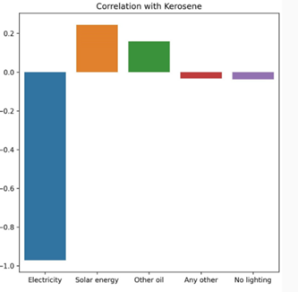
We fond a negative correlation between Households using electricity and those using Kerosene - which implies less reliance on Kerosene as electricity distribution increases.
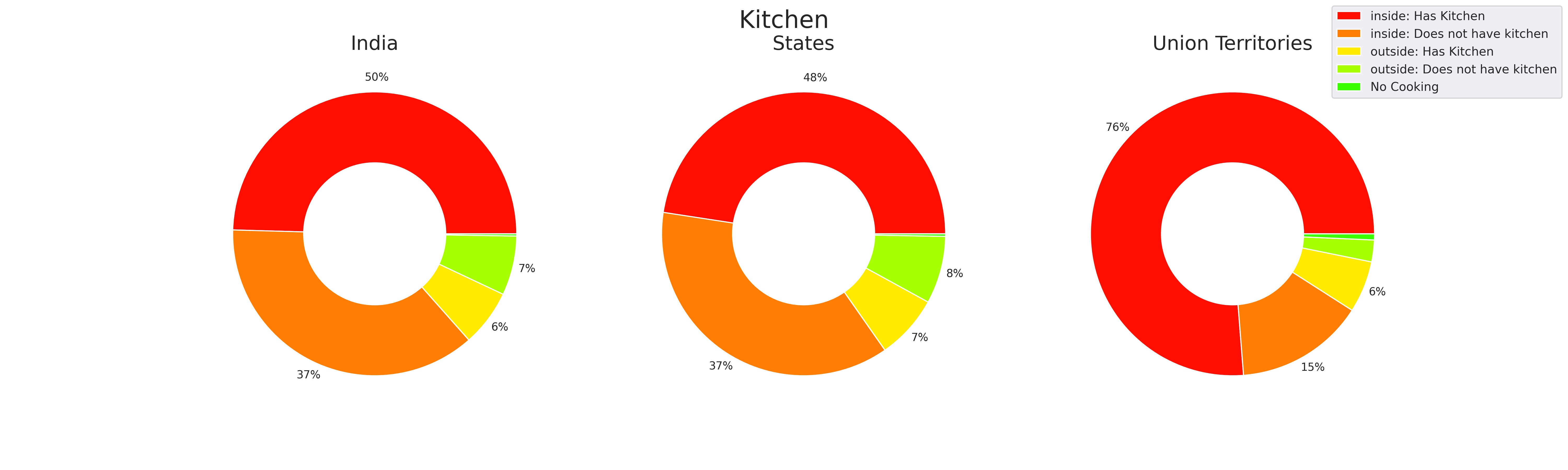
The union territories had much better kitchen facilities compared to the other states of India and India as a whole.
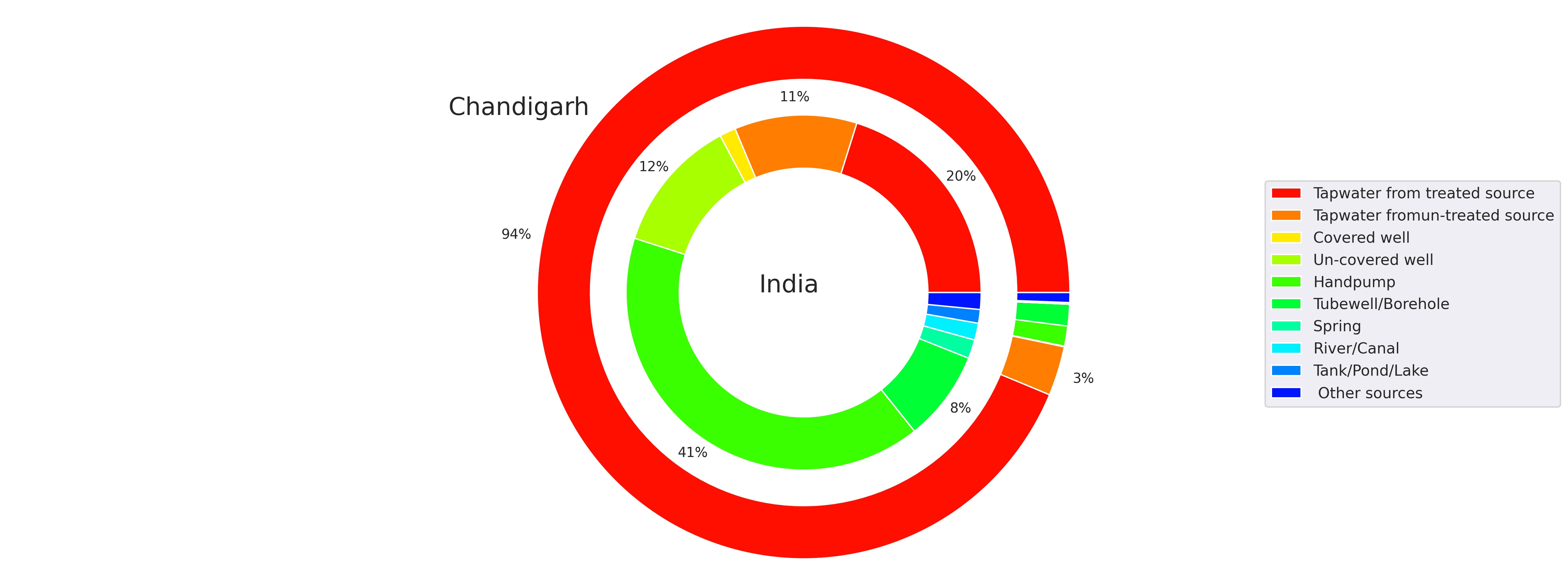
While comparing each facility of a state against the country average, some states like Chandigarh, have much better water facilities than India as a whole.
On Comparing the distribution of the facility across the country, Bihar, Assam, Jharkhand, Meghalaya, Uttar Pradesh and Odisha heavily rely on Kerosene.
Two filtering algorithms are built to answer a question What state should I live in?. The principle of both the algorihtms are same, filter the states on the basis of their basic amenities and characteristics and provvide end user the results. The difference is in the results algorithm 1 gives us the count of districts in state where there are availibiity of certain amenity satisfies the user defined threshold. Algorithm 2 provides us with visualizatios of mean percentage availibility of the assets selected by the users. Algorithm 2 can be observed in the UI and Algorithm 1 can be found in the PART A folder.
Exmaples
Algorithm 1: If a user wants to live in an owned house with wooden roof with threshold of 50, wooden walls with threshold of 50, indoor bathroom with threshold of 50, drinkable, tap water with threshold of 20, the statewise count of places is returned and shown below:
Algorithm 2: A user selects 'Facilities to choose' to choose from the main column, then a select box named Choose further from Lighting source appears where we select 'Kerosene for lighting' in the first case and 'Electricity for lighting' in the second one. The maps generated are present here for comparison between the distribution of two ameneties:
You can also tweak the plot size and the number of enteries in the plot by using the sliders provided.
The data set is an open source data set available at kaggle. The data contains information about the house and its amenities as mentioned above. The data is distributed in 5 files and each represent a metro city. Delhi, Mumbai, Bangalore, Chennai, Hyderabad and Kolkata are the ones that are present in the data. Price is our target variable and the rest 39 variables are accounted as feature variables.
In level1 we create the master data by combining the files for the six cities. This operation is carried out using pandas concat method with ignoring the indexes of the original datasets so to define a unified index, to disregard the problem of duplicate indices. This ensures that queries on the data set is run smoothly and correctly. This aggregated data is what we are calling the master data. The master data is then split into training and test set which acts an input for level2. The distribution of the dependent variable Price is highly left skewed which makes certain estimates on it very unrelaible, hence we model on the log transformation of the dependent variable. The log transformation brings the distribution closer to a normal distribution and also scales range of the variable. The effect of log transformation are on the dependent variable is shown below.

• Drops Unecessary Columns: The drop columns operation is a custom class in our pipeline which takes a list of columns and drop them from the dataset.
• Replace NaN Values: The null values in the binary features is represented by the digit 9, this operation finds those values and replace them with Nan(Not a Number)
• Add Area Bins: This is one of the feature engineering operations that we do in our pipeline. It evalutes the quantiles of the feature Area and assigns the corresponding quantile number(1, 2, 3, 4) in which a sample resides. This provides a relative information of the size of a house and we call this new variable AreaType; small if it resides in quantile 1 encoded as 1, medium if it resides in quantile 2 encoded as 2, large if it resides in quantile 3 encoded as 3 and very large if it resides in quantile 4 encoded as 4.
• Custom Imputer: This is one of the most important operation of this pipeline, imputing the null/NaN values. We came up with a better solution than just imputing the null values with most frequent classes in the in dataset for each feature. Our custom imputer uses the relative area information using the area bins created earlier.
• Handle Outliers: In this operation we handle the outliers in feature Area as shown above on the right of Figure 1 by replacing the outliers with by Q1-1.5IQR and Q3+1.5IQR, where Q1, Q2 and IQR is the 25th percentile, 75th percentile and Interquartile range respectively; any things less than Q1-1.5IQR is reassigned as Q1-1.5IQR and any value greater than Q3+1.5IQR to Q3+1.5IQR.
• One Hot Encoder: One hot encoding is extensively used in encoding categorical columns to series of binary dummy columns, one for each category in which 0 represents that a sample does not correspond to the class where as 1 represent that a sample represent to this particular class.
• Feature Engineering: Though we have done some feature engineering above but this is the more advanced one as we augment our data with the Indian Housing Census Data 2011. Our aim is to add Housing Quality of Living Index(HQLI) for each state in our dataset. It depends upon three variables which are quality of housing index(QHI), basic amenity index(BAI), asset index(AI). HQLI = QHI + BAI + AI.
• Standardization: We standardize our continious features using this operation, Standardization comes into picture when features of input data set have large differences between their ranges, or simply when they are measured in different measurement units. We take down the mean of the distribution to zero and the standard deviation to 1, stabalizing the variance and the learning process
• Linear Regression
• K-Nearest Neighbors
• Neural Network
• Decision Tree
• Bagging Ensembles
• Random Forest
• Gradient Boosting Algorithms
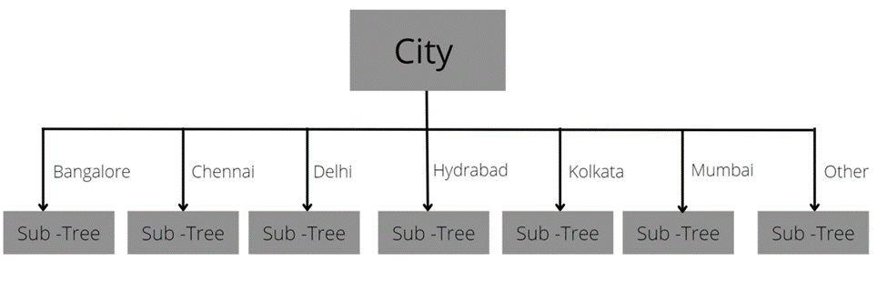
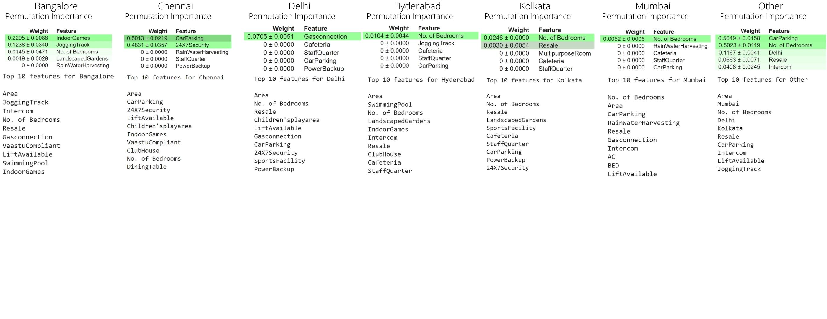
Through this model we ensure that the highest importance is given to the city in which the house is located in. From our analysis we know that the highest importance is given to features which represent city like mumbai, kolkata, etc. This model also considers the fact that a house cannot be in 2 cities at once. for example, any record cannot contain Bangalore=1 and Chennai=1 as well (unless it is a mistake in which case the decision tree will traverse to sub-tree under the 'Other' branch). So in this approach we divided the training data according to city. We will then train 6 decision trees for all the cities present in the training data. We also train a 7th decision tree on the whole training dataset so that if the test dataset contains a record of a house in a new city(city which is not in training) then the model can still predict for that record. We then aggregated all our results into a list and then found our mean squared error and R2 score for train data as well as test data.
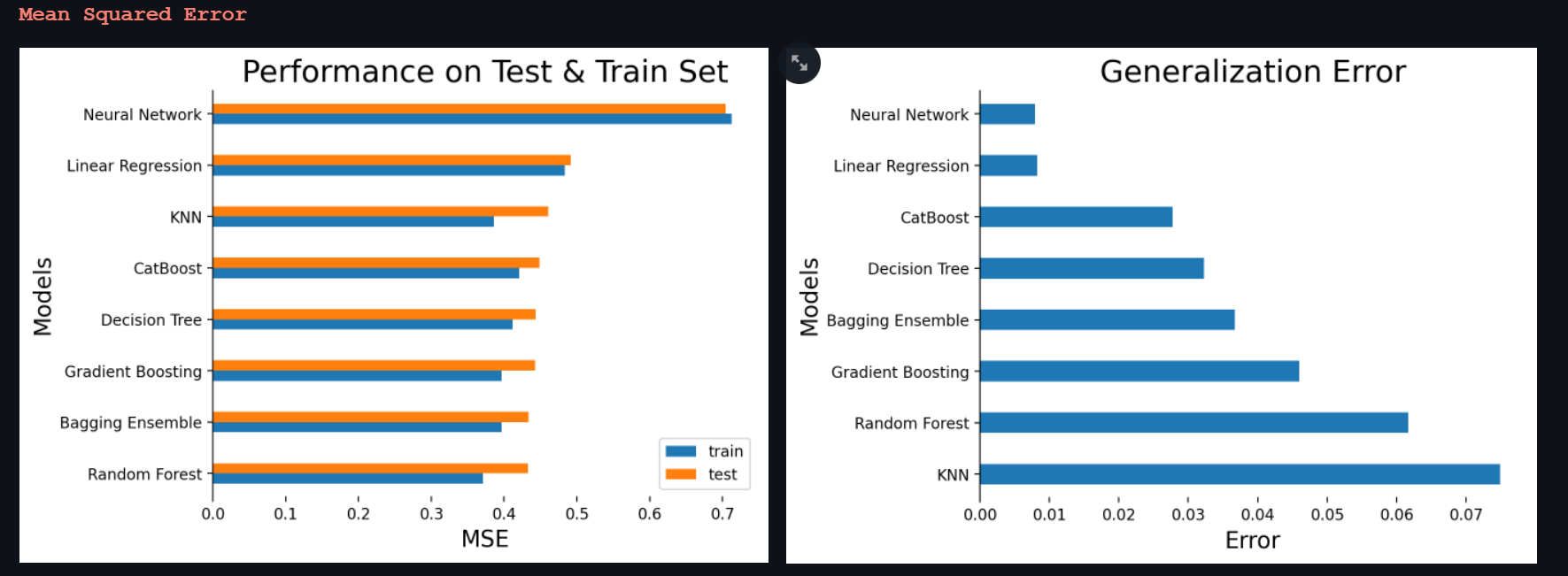
Random forest outperforms every other model in terms of test mse while the most complex network in the kitty; the neural network has the worst mse on the test set. The above graph is sorted with respect to the test set mse. The generalization error is the difference between the mse of train set and test set. Random forest seems to generalise poorly as compared to other models with higher mse.
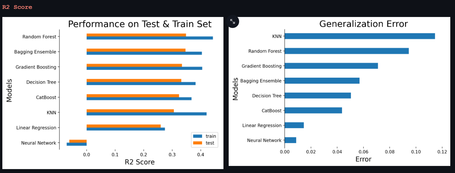
Neural Network again the worst performer and is not able to explain any variance of the features in the predictions. The Random Forest does bag the highest rank but again the generalization error is quite high, in comparison, bagging ensemble looks more robust as the generalization is low and test mse and r2score are similar to that of Random Forest. Since the bagging model is more robust we choose the bagging model as our best performing model.

FEATURE IMPORTANCE
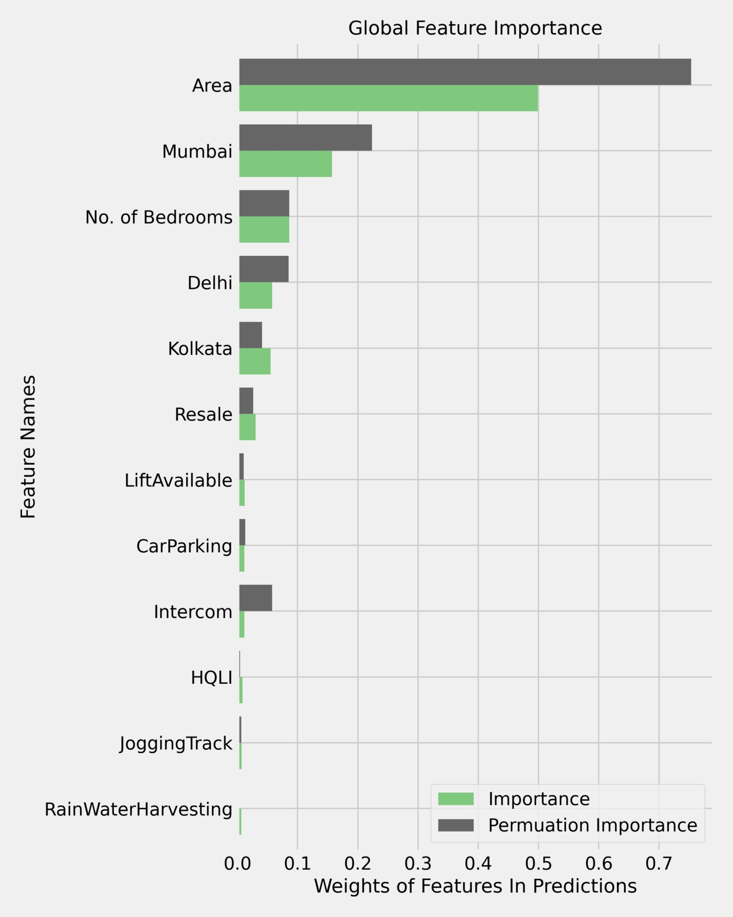
The above figure conveys the feature importance calculated as the average decrease in variance in the bagging ensemble shown in green and permuation feature importance calculated by permuting a feature column at once and noticing the drop in the oberving metrics shown in grey. These are the top 12 features who contributes gloabally in a predictions, the impact of the rest are negligible. Area is an expected feature to pop up in such metrics and has been ranked the top most feature that contributes globally in making predictions. It is interesting to see that onehot encoded variables for cities are considered importance as well which do indicate that the model is learning from the trend of prices in each city. Number of bedrooms has also made it place and it makes sense as that the price a house with more bedroom is more than a house with less number of bedrooms. Resale, availability of car parking and intercom are also key factors. The engineered feature HQLI has a relatively higher importance to the 30 or more features below it. Rain water harvesting is interesting to see in the mix.
LIME INFERENCES CAN BE FOUND ON OUR WEB APP REPORT, here : https://share.streamlit.io/aamir09/ds2project/main/app/app.py
FEATURE IMPORTANCE
The Feature Importance and Permutation Importance of all 7 decision trees are as given below:
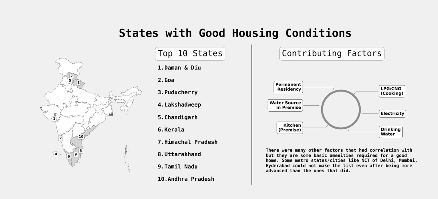
While working on this project, we learnt so much about the diversity that we have in India. Union Territories and small states like Daman & Diu, Chandigarh and Goa had better facilities than the big metro cities in India. The exploeratory data analysis does justify the phrase it is not what it looks like as we gathered so many interesting facts about the country. The housing data was in itself a challenge with all the null values it had but at the end, we were able to get pretty decent results and explainable models.
[1] When and Why to Standardize Your Data?, https://builtin.com/data-science/when-and-why-standardize-your-data
[2] K-nearest Neighbours Regression, https://bookdown.org/tpinto_home/Regression-and-Classification/k-nearest-neighbours-regression.html
[3] Neural Network, https://www.investopedia.com/terms/n/neuralnetwork.asp
[4] Decision Trees for Classification: A Machine Learning Algorithm, https://www.xoriant.com/blog/product-engineering/decision-trees-machine-learning-algorithm.html
[5] Gradient boosting machines, a tutorial, https://www.frontiersin.org/articles/10.3389/fnbot.2013.00021/full
[6] What is Local Interpretable Model-Agnostic Explanations (LIME)?, a tutorial, https://c3.ai/glossary/data-science/lime-local-interpretable-model-agnostic-explanations/
- Scraping-Housing data.ipynb - We start by scraping the Census data from the website, then in order to get a 'per capita' understanding of the census we scrape Indian population data. Next we scrape latitude and longitude data for every district in the data in order to be used in the web app
- eda1.ipynb - In this notebook, we have compared the facilities in the states and Union territories vs the country. We have also seen the top-5 states for each feature, and the situation of the country as a whole. We have marked the top and bottom ranked states in each feature, and plotted the correlation matrix of living conditions with other features as well.
- eda2.ipynb - The notebook provides answers to some interesting questions about the state of housing in India. The notebook contains infographics as well as self explanatory graphs to visualize the findings. At the end of the notebook the process of generating QHI, BAI and AI cvs's is also mentioned.
- eda3.ipynb - We try to answer some questions regarding the basic necessities of Indian households e.g Distribution of Electricity, toilet facilities
- filterAlgorithm1 - Filter the states on the basis of their basic amenities and characteristics and provvide end user the results. It gives us the count of districts in state where there are availibiity of certain amenity satisfies the user defined threshold.
- stateRankings.ipynb - Here, we have ranked the best states and the worst states for living based on the features in the Household census data. We have given weights to each feature and calculated it using standardized scores and well as normalized scores.
- Models - This folder contains files used to build the machine learning and deep learning models in our pipeline.
- Datasets - This folder contains datasets for creating the master data.
- main.py - It creates the master data, pipelines and generates results on the test results. To recreate our pipeline results: a) Clone the repository b) Open in VS Code c) Open a new terminal and make sure you have the required libraries d) Run Command: python PartB/main.py
- pipelineClasses.py - It contains all the classes used in our pipeline. The file is well documented.
- createMasterData.py - It contains code to create master data which we use in the file main.py.
- approachBModel.ipynb- It contains code and results for approach B.
- AI, BAI, QHI - These CSV files are used to generate HQLI feature and are used in pipelineClasses.py file.
- Notebook1.ipynb , Notebook2.ipynb - The notebooks are in the raw state, containing all the experiments done while creating the pipeline.
- Noteboo3_creating_dataframes - This notebook contains the steps followed to create sub data frames for each super column of 2011 Indian Housing Census Data.
- app.py - This py file contains code for our streamlit report app.
- images - This folders contains all the images used in our streamlit report.
- requirements.txt - The file is used to install required libraries in streamlit.
These are the train and test data generated from the pipelines made available for the public to use in their modelling.
The data is the master data generated which contains no alterations from our pipeline. It is the concatenation of all the states and created with the file createMasterData.py in PART B.