LLM from Scratch — Hands-On Curriculum (PyTorch)

Part 0 — Foundations & Mindset

• 0.1 Understanding the high-level LLM training pipeline (pretraining → finetuning → alignment)
• 0.2 Hardware & software environment setup (PyTorch, CUDA/Mac, mixed precision, profiling tools)

conda create -n llm_from_scratch python=3.11
conda activate llm_from_scratch
pip install -r requirements.txt

Part 1 — Core Transformer Architecture

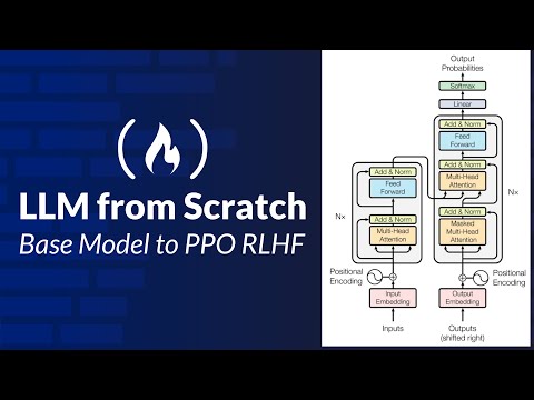
• 1.1 Positional embeddings (absolute learned vs. sinusoidal)
• 1.2 Self-attention from first principles (manual computation with a tiny example)
• 1.3 Building a single attention head in PyTorch
• 1.4 Multi-head attention (splitting, concatenation, projections)
• 1.5 Feed-forward networks (MLP layers) — GELU, dimensionality expansion
• 1.5 Residual connections & LayerNorm
• 1.6 Stacking into a full Transformer block

Part 2 — Training a Tiny LLM

• 2.1 Byte-level tokenization
• 2.2 Dataset batching & shifting for next-token prediction
• 2.3 Cross-entropy loss & label shifting
• 2.4 Training loop from scratch (no Trainer API)
• 2.5 Sampling: temperature, top-k, top-p
• 2.6 Evaluating loss on val set

Part 3 — Modernizing the Architecture

• 3.1 RMSNorm (replace LayerNorm, compare gradients & convergence)
• 3.2 RoPE (Rotary Positional Embeddings) — theory & code
• 3.3 SwiGLU activations in MLP
• 3.4 KV cache for faster inference
• 3.5 Sliding-window attention & attention sink
• 3.6 Rolling buffer KV cache for streaming

Part 4 — Scaling Up

• 4.1 Switching from byte-level to BPE tokenization
• 4.2 Gradient accumulation & mixed precision
• 4.3 Learning rate schedules & warmup
• 4.4 Checkpointing & resuming
• 4.5 Logging & visualization (TensorBoard / wandb)

Part 5 — Mixture-of-Experts (MoE)

• 5.1 MoE theory: expert routing, gating networks, and load balancing
• 5.2 Implementing MoE layers in PyTorch
• 5.3 Combining MoE with dense layers for hybrid architectures

Part 6 — Supervised Fine-Tuning (SFT)

• 6.1 Instruction dataset formatting (prompt + response)
• 6.2 Causal LM loss with masked labels
• 6.3 Curriculum learning for instruction data
• 6.4 Evaluating outputs against gold responses

Part 7 — Reward Modeling

• 7.1 Preference datasets (pairwise rankings)
• 7.2 Reward model architecture (transformer encoder)
• 7.3 Loss functions: Bradley–Terry, margin ranking loss
• 7.4 Sanity checks for reward shaping

Part 8 — RLHF with PPO

• 8.1 Policy network: our base LM (from SFT) with a value head for reward prediction.
• 8.2 Reward signal: provided by the reward model trained in Part 7.
• 8.3 PPO objective: balance between maximizing reward and staying close to the SFT policy (KL penalty).
• 8.4 Training loop: sample prompts → generate completions → score with reward model → optimize policy via PPO.
• 8.5 Logging & stability tricks: reward normalization, KL-controlled rollout length, gradient clipping.

Part 9 — RLHF with GRPO

• 9.1 Group-relative baseline: instead of a value head, multiple completions are sampled per prompt and their rewards are normalized against the group mean.
• 9.2 Advantage calculation: each completion’s advantage = (reward – group mean reward), broadcast to all tokens in that trajectory.
• 9.3 Objective: PPO-style clipped policy loss, but policy-only (no value loss).
• 9.4 KL regularization: explicit KL(π‖π_ref) penalty term added directly to the loss (not folded into the advantage).
• 9.5 Training loop differences: sample k completions per prompt → compute rewards → subtract per-prompt mean → apply GRPO loss with KL penalty.