There are data with binary classes and data with various classes in the world. Finding a classifier that perfectly distinguishes classes for these data is a key task in classification problems. However, it is a very difficult problem to find linear classifiers just for data with binary classes, not to mention multi-class data. This tutorial contains the contents of kernel-based learning for the purpose of discovering the classifier. In this tutorial, support vector machine and support vector regression are described as the methodology of kernel-base learning. In addition, various hyperparameters are adjusted for various datasets, and analysis of experimental results is the main content.
The table of contents is as follows.
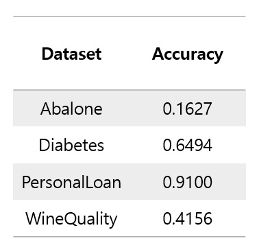
We use 4 classification datasets for SVM (abalone, Diabetes, PersonalLoan, WineQuality)
We use 3 regression datasets for SVR (Concrete, Estate, ToyotaCorolla)
abalone dataset : https://www.kaggle.com/datasets/rodolfomendes/abalone-dataset
Diabetes dataset : https://www.kaggle.com/datasets/mathchi/diabetes-data-set
PersonalLoan dataset : https://www.kaggle.com/datasets/teertha/personal-loan-modeling
WineQuality datset : https://www.kaggle.com/datasets/uciml/red-wine-quality-cortez-et-al-2009
Concrete dataset : https://www.kaggle.com/datasets/elikplim/concrete-compressive-strength-data-set
Estate dataset : https://www.kaggle.com/datasets/arslanali4343/real-estate-dataset
ToyotaCorolla dataset : https://www.kaggle.com/datasets/klkwak/toyotacorollacsv
In all methods, data is used in the following form.
import argparse

def Parser1():
    parser = argparse.ArgumentParser(description='1_Dimensionality Reduction')

    # data type
    parser.add_argument('--data-path', type=str, default='./data/')
    parser.add_argument('--data-type', type=str, default='abalone.csv',
                        choices = ['abalone.csv', 'BankNote.csv', 'PersonalLoan.csv', 'WineQuality.csv', 'Diabetes.csv', 'Concrete.csv',
                                    'Estate.csv', 'ToyotaCorolla.csv'])

data = pd.read_csv(args.data_path + args.data_type)

X_data = data.iloc[:, :-1]
y_data = data.iloc[:, -1]
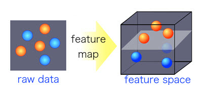
In general, Support Vector Machine refers to a methodology for separating data using a line called a 'Hyperplane'.
However, in the case of the above picture, it is possible to create a lot of hyperplanes that separate the data well just by properly changing the slope of the line.
Accordingly, there may be a question of which hyperplane is the optimal hyperplane.
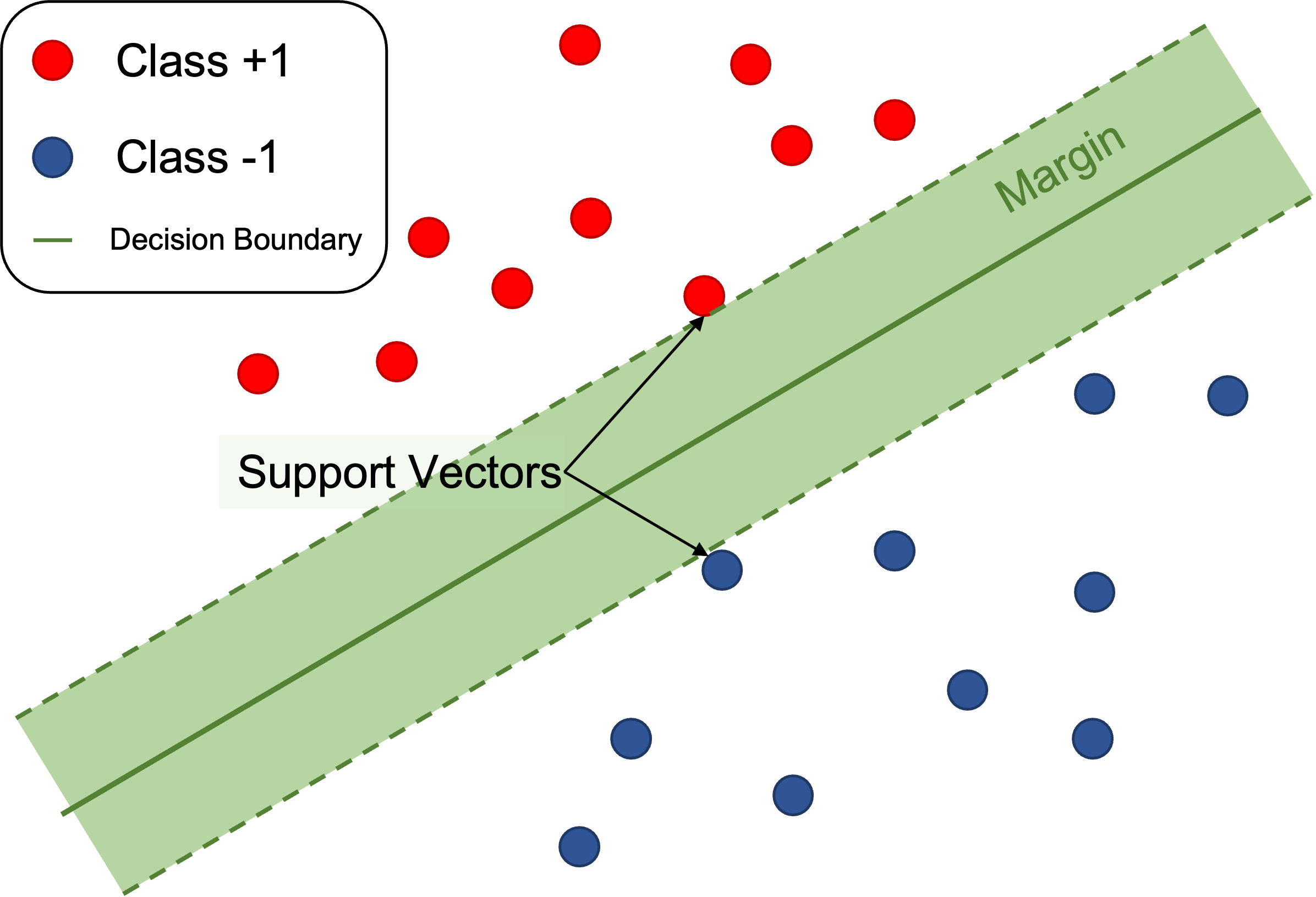
As shown in the picture below, SVM uses the hyperplane that maximizes 'Margin' as the optimal hyperplane.
However, data that is completely linearly separated like the data above, as you may have noticed, rarely exists in reality.
Therefore, in general, some errors are allowed, non-linear classifiers are used, and non-linear classifiers and errors are used simultaneously.
Arrange each case in the table of contents below.

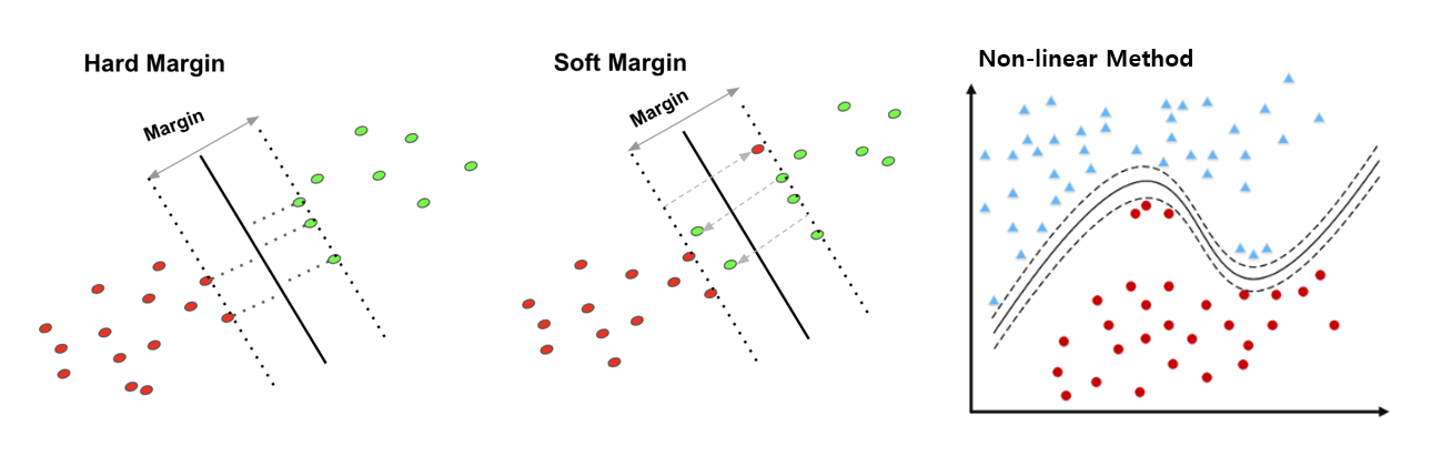
The first case, Linearly Hard Margin, is a very basic form of SVM. This method assumes that the data is linearly separated and has a feature that does not allow any errors. As mentioned above, it can be said that it is a very difficult method to apply in reality.
The second case, Linearly Soft Margin, is a method of maintaining a linear classifier shape but allowing a certain amount of error. How much error is allowed can be set through the "C" value, which is a hyperparameter, and the performance difference according to the "C" value will be verified in the 'Analysis' table of contents later.
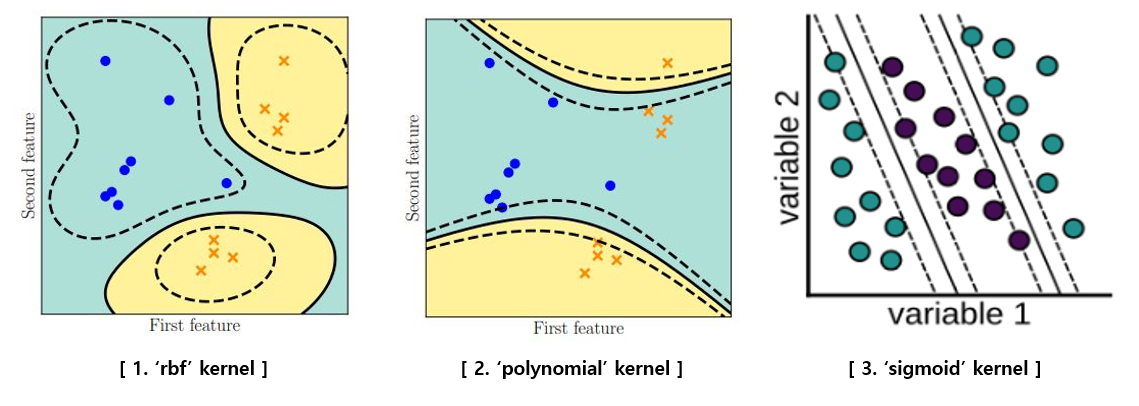
Thr fourth case(we do not care third case), Non-linearly Soft Margin, The fourth method is a non-linear method that applies a soft margin method that allows errors and uses a non-linear mapping technique to map on a high-dimensional space. We compare the performance according to the 'rbf' method and the 'polynomial' method, which are widely known non-linear methods in later experiments.
import numpy as np
import pandas as pd
import matplotlib.pyplot as plt
from sklearn import svm

from sklearn.preprocessing import MinMaxScaler
from sklearn.model_selection import train_test_split
from sklearn.metrics import accuracy_score

def Linearly_Hard_Case(args):
    data = pd.read_csv(args.data_path + args.data_type)
    h = .02
    X_data = data.iloc[:, :-1]
    y_data = data.iloc[:, -1]
    scaler = MinMaxScaler()
    X_scaled = scaler.fit_transform(X_data)

    X_train, X_test, y_train, y_test = train_test_split(X_scaled, y_data, test_size = args.split_size, shuffle=True, random_state = args.seed)

    clf = svm.SVC(kernel='linear') # 1e-10 means very small value which is close to "0" (There's no Hard-margin method in sklearn)
    clf.fit(X_train, y_train)
    print('Training SVM : Linearly-Hard Margin SVM.....')

    # Prediction
    pred_clf = clf.predict(X_test)
    accuracy_clf = accuracy_score(y_test, pred_clf)
    print('Linearly-Hard margin SVM accuracy : ', accuracy_clf)
We used the scikit-learn package to implement SVM. To implement first case, Linearly-Hard case, we set the hyperparameter 'C' as 1e-10, which is close to "0". In the scikit-learn method, this method was used because the C value could not be set to 0.
In the case of the first case, Linearly Hard Margin, there is no specific hyperparameter to tune for performance comparison. Therefore, hyperparameter tuning for performance comparison will be performed in the second and third cases.
For visualization, two X variables were extracted from each dataset to learn, and the data and linear classifier were visualized.
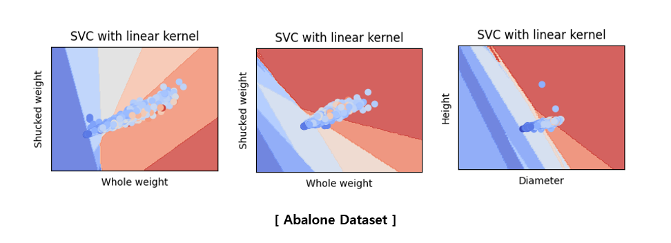
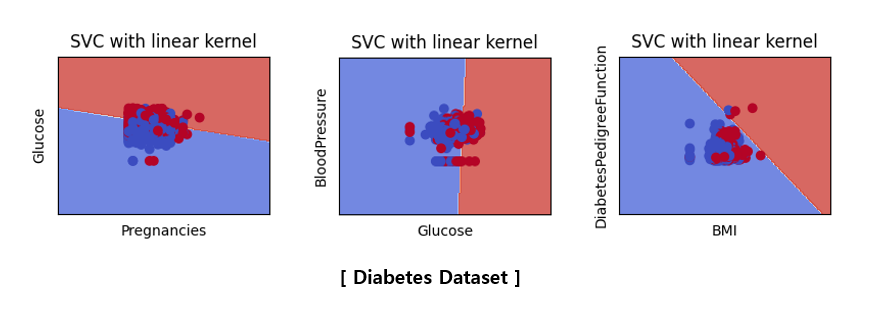
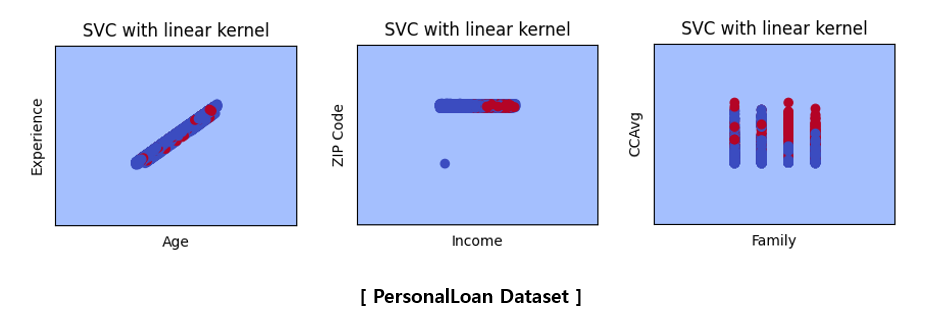
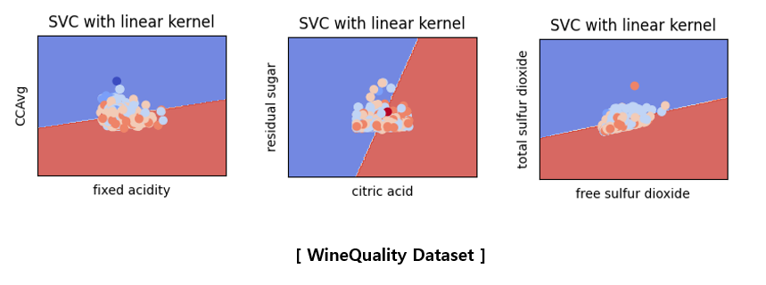
The above pictures are not related to the accuracy score table shown earlier because they are the results of learning by selecting only two variables. Since only two variables were used, the classification accuracy is very poor and the characteristics of the data are not accurately described. To visualize what happens when SVM is applied instead of hyperparameter tuning, only two variables were used to plot in a two-dimensional space. It would be good to think of it as a reference material that visually understands that SVM proceeds in this way.
import numpy as np
import pandas as pd
import matplotlib.pyplot as plt
from sklearn import svm

from sklearn.preprocessing import MinMaxScaler
from sklearn.model_selection import train_test_split
from sklearn.metrics import accuracy_score

def Linearly_Soft_Case(args):
    data = pd.read_csv(args.data_path + args.data_type)

    X_data = data.iloc[:, :-1]
    y_data = data.iloc[:, -1]

    scaler = MinMaxScaler()
    X_scaled = scaler.fit_transform(X_data)

    X_train, X_test, y_train, y_test = train_test_split(X_scaled, y_data, test_size = args.split_size, shuffle=True, random_state = args.seed)

    clf = svm.SVC(C = args.C, kernel='linear') # C is bigger than 0 because error is allowed.
    clf.fit(X_train, y_train)
    print('Training SVM : Linearly-Soft Margin SVM.....')

    # Prediction
    pred_clf = clf.predict(X_test)
    accuracy_clf = accuracy_score(y_test, pred_clf)
    print('Linearly-Soft margin SVM accuracy : ', accuracy_clf)
If the C value is used as a very small number close to zero in the first case, the C value is set as a hyperparameter because the error is allowed in the second case. In the second case, we conducted a comparative experiment on how the performance changes according to the value of hyperparameter C.
Before we do analysis, let's talk about the hyperparameter 'C'. Hyperparameter C can be said to be a value that adjusts how much error is allowed in the Softmargin SVM that allows error. It is difficult to explain in words, so it is good to refer to the formula below.
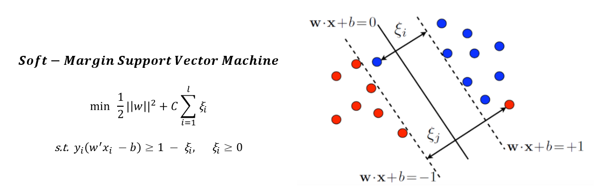
Looking at the optimization formula, it is a problem of minimization for the overall equation, and the right term has a product of the sum of the error term and C. Therefore, if the C value is taken high, the sum of the error terms will be induced to have a small value for the purpose of minimization. Conversely, if the C value is low, it indicates that the error term will be allowed relatively more than if the C value is high. We will look at the following Analysis Table of Contents to see how performance changes according to changes in C values.

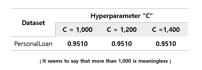
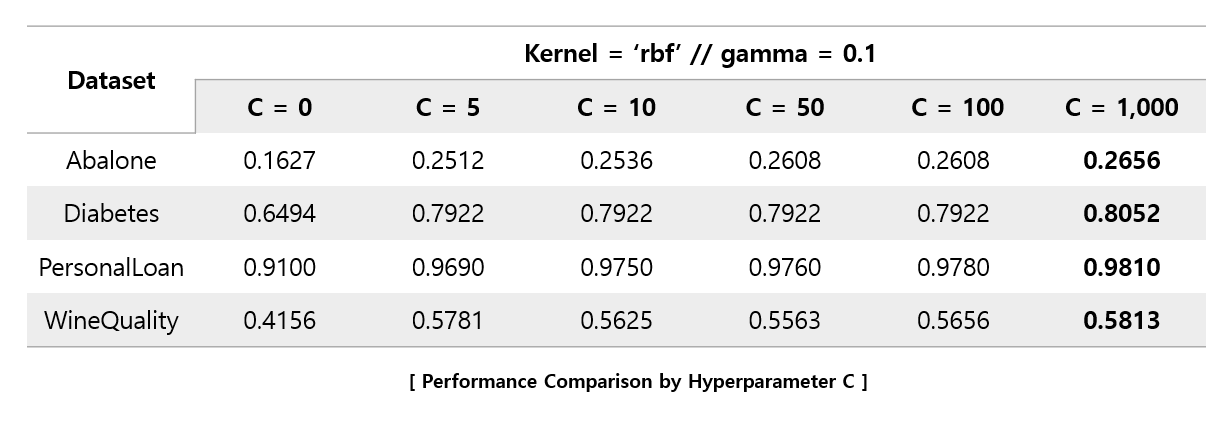
As you can see, excluding PersonalLoan dataset, increasing the C value does not mean improving performance. This can be interpreted that if the C value becomes appropriately large, the magnitude of the error to be multiplied with the C value converges to almost zero, so that the C value does not affect the performance. It can be seen that most datasets converge to a specific accuracy value as the C value increases. And most of them performed best when the C value was 5 or 10, but PersoanlLoan's performance continued to rise as the C value increased. So, we checked whether the performance converges when the PersonalLoan dataset has a C value.
import numpy as np
import pandas as pd
import matplotlib.pyplot as plt
from sklearn import svm

from sklearn.preprocessing import MinMaxScaler
from sklearn.model_selection import train_test_split
from sklearn.metrics import accuracy_score

def Non_linearly_Soft_Case(args):
    data = pd.read_csv(args.data_path + args.data_type)

    X_data = data.iloc[:, :-1]
    y_data = data.iloc[:, -1]

    scaler = MinMaxScaler()
    X_scaled = scaler.fit_transform(X_data)

    X_train, X_test, y_train, y_test = train_test_split(X_scaled, y_data, test_size = args.split_size, shuffle=True, random_state = args.seed)

    clf = svm.SVC(C = args.C, kernel = args.kernel) # C is bigger than 0 because error is allowed.
    clf.fit(X_train, y_train)
    print('Training SVM : Non_linearly-Soft Margin SVM with ' + args.kernel + '.....')

    # Prediction
    pred_clf = clf.predict(X_test)
    accuracy_clf = accuracy_score(y_test, pred_clf)
    print('Non_linearly-Soft margin SVM with ' + args.kernel + 'accuracy : ', accuracy_clf)
Similarly, there is no significant difference in code, but kernel is used as one of the following three rather than linear.
 Interestingly, all four datasets performed best at 1,000, the maximum value of C set. In addition, we re-experimented by increasing the C value further.
 When the C value exceeded 1,200, the performance converged, and rather, a falling dataset was found. For the four datasets, it was found that the C values of 1,000 to 1,200 showed the best performance.
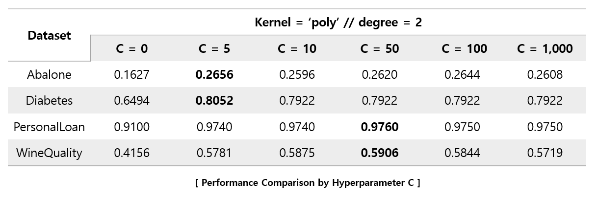
In the case of using the 'Polynomial' kernel, it can be seen that the performance decreases significantly as the C value approaches 1,000. Unlike when using the 'rbf' kernel, it can be seen that the C value forms an optimal value between 5 and 50.
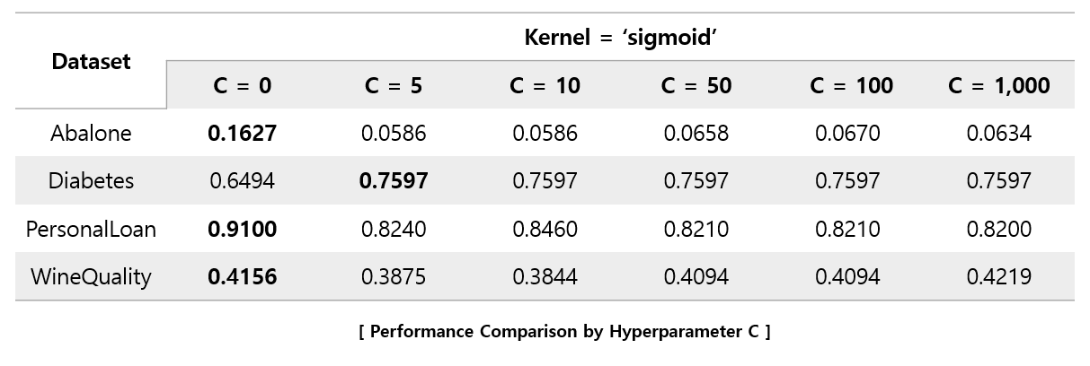
In the case of the 'sigmoid' kernel, it can be seen that as the C value increases, the performance rather degrades.
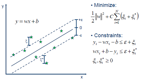
When the regression equation is estimated, the SVR generates 2ϵ(−ϵ,ϵ)tubes above and below the regression equation. As you know, the regression problem is almost impossible to predict the exact value. So, if there is an actual value in the tube, the penalty is given as 0 to tolerate even if there is a difference from the predicted value. If there is an actual value outside the tube, it is given penalty at the magnification of C. It's kind of giving a kind of upper, lower limit for the regression line of regression. In summary, SVR assumes that there is noise in the data and does not seek to fully estimate the noisy real value considering these points, thus allowing the difference between the real value and the predicted value within a reasonable range.
import numpy as np
import pandas as pd
import matplotlib.pyplot as plt
from sklearn import svm
from sklearn.preprocessing import MinMaxScaler
from sklearn.model_selection import train_test_split
from sklearn.metrics import mean_squared_error, r2_score, mean_absolute_percentage_error
def SVR(args):
data = pd.read_csv(args.data_path + args.reg_data)
X_data = data.iloc[:, :-1]
y_data = data.iloc[:, -1]
scaler = MinMaxScaler()
X_scaled = scaler.fit_transform(X_data)
X_train, X_test, y_train, y_test = train_test_split(X_scaled, y_data, test_size = args.split_size, shuffle=True, random_state = args.seed)
if args.kernel == 'rbf':
clf = svm.SVR(C = args.C, kernel = args.kernel, gamma = args.gamma) # C is bigger than 0 because error is allowed.
clf.fit(X_train, y_train)
print('Training SVR with ' + args.kernel + '.....')
elif args.kernel == 'poly':
clf = svm.SVR(C = args.C, kernel = args.kernel, degree = args.degree) # C is bigger than 0 because error is allowed.
clf.fit(X_train, y_train)
print('Training SVR with ' + args.kernel + '.....')
else:
clf = svm.SVR(C = args.C, kernel = args.kernel) # C is bigger than 0 because error is allowed.
clf.fit(X_train, y_train)
print('Training SVR with ' + args.kernel + '.....')
# Prediction
pred_clf = clf.predict(X_test)
reg_r2_score = r2_score(y_test, pred_clf)
reg_mae_score = mean_squared_error(y_test, pred_clf)
reg_mape_score = mean_absolute_percentage_error(y_test, pred_clf)
print('SVR with ' + args.kernel + 'R2 Score : ', reg_r2_score)
print('SVR with ' + args.kernel + 'MAE Score : ', reg_mae_score)
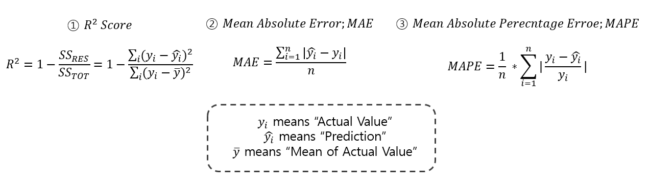
print('SVR with ' + args.kernel + 'MAPE Score : ', reg_mape_score)Unlike SVM, SVR is a regression problem, so the metrics must be changed. So, we used three metrics, R2_score, Mean Absolute Error, and Mean Absolute Percent Error, instead of using existing accuracy metrics. The formula for evaluation indicators is briefly shown below.
The SVR can utilize a linear kernel. And also, as in the case of Non-linearly Soft Margin, SVR also utilizes a non-linear kernel. Likewise, 'rbf', 'poly', were used(Sigmoid kernels quite do not fit well, so totally 3-kernels were used).
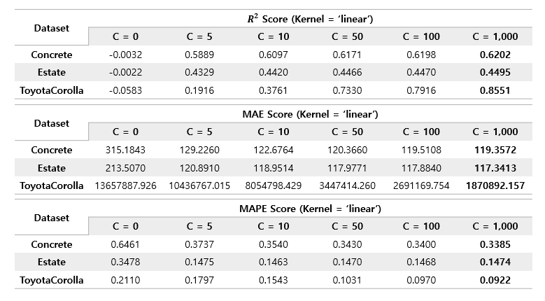
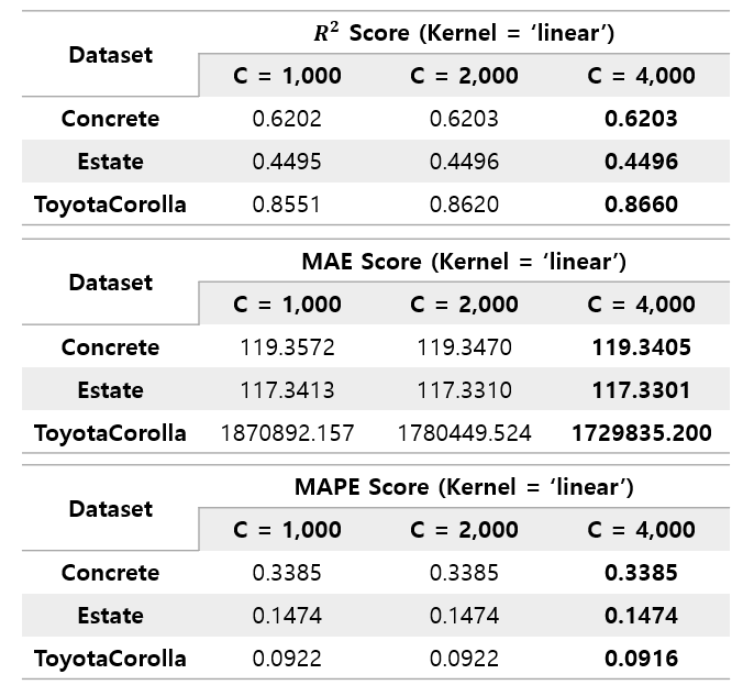
Likewise, rbf's performance improved as C increased to a value of 1000, and the increase in performance was much larger than that of linear kernel. Similarly, C was re-experimented by increasing it to 4000.
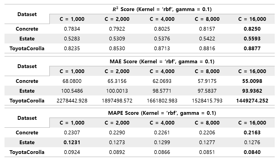
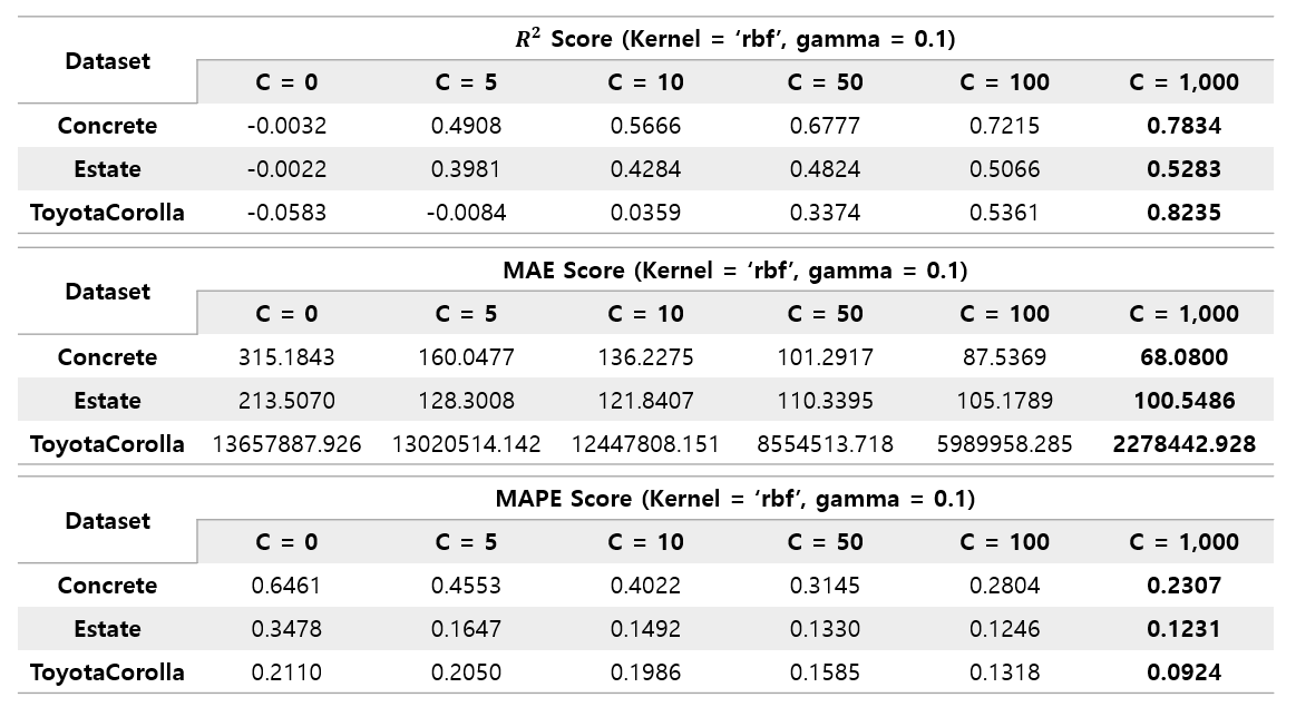
The C value was intended to be up to 4000, but the performance continued to rise to 16000. Through this, it was found that the threshold of the C value, in which performance improvement continues, was different for each kernel.
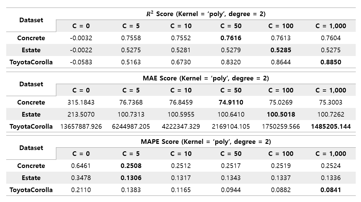
The poly kernel showed a different pattern from the previous two kernels. Concrete dataset and Estate dataset showed that their performance almost converged even when the C value was only 5~10. And in the case of Toyota Corolla dataset, even if the C value was not raised to 16000 like the previous rbf kernel, it already showed the best performance in all three kernels at about 1000. However, the convergence values of Concrete and Estate datasets were not the best performance, and these datasets performed best when using rbf kernel.
As a result, it was found that the types of kernels that extract good performance are different for each dataset.