EHN: True Velocity in Convection Maps#307
Conversation
|
Matplotlib version= 3.5.3 import matplotlib.pyplot as plt map_file = "20110128.north.map2" plt.figure(figsize=(8,6)) plt.figure(figsize=(8,6))
|
|
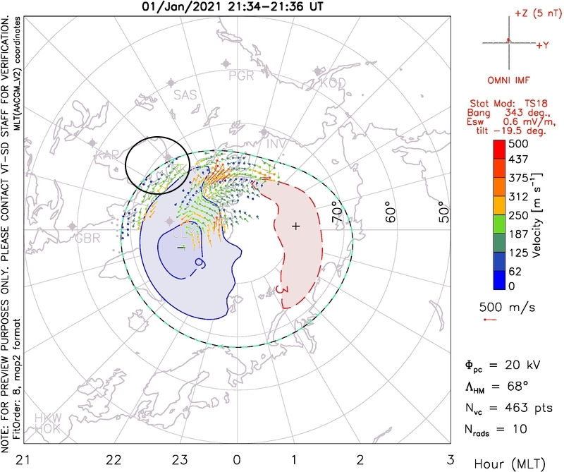
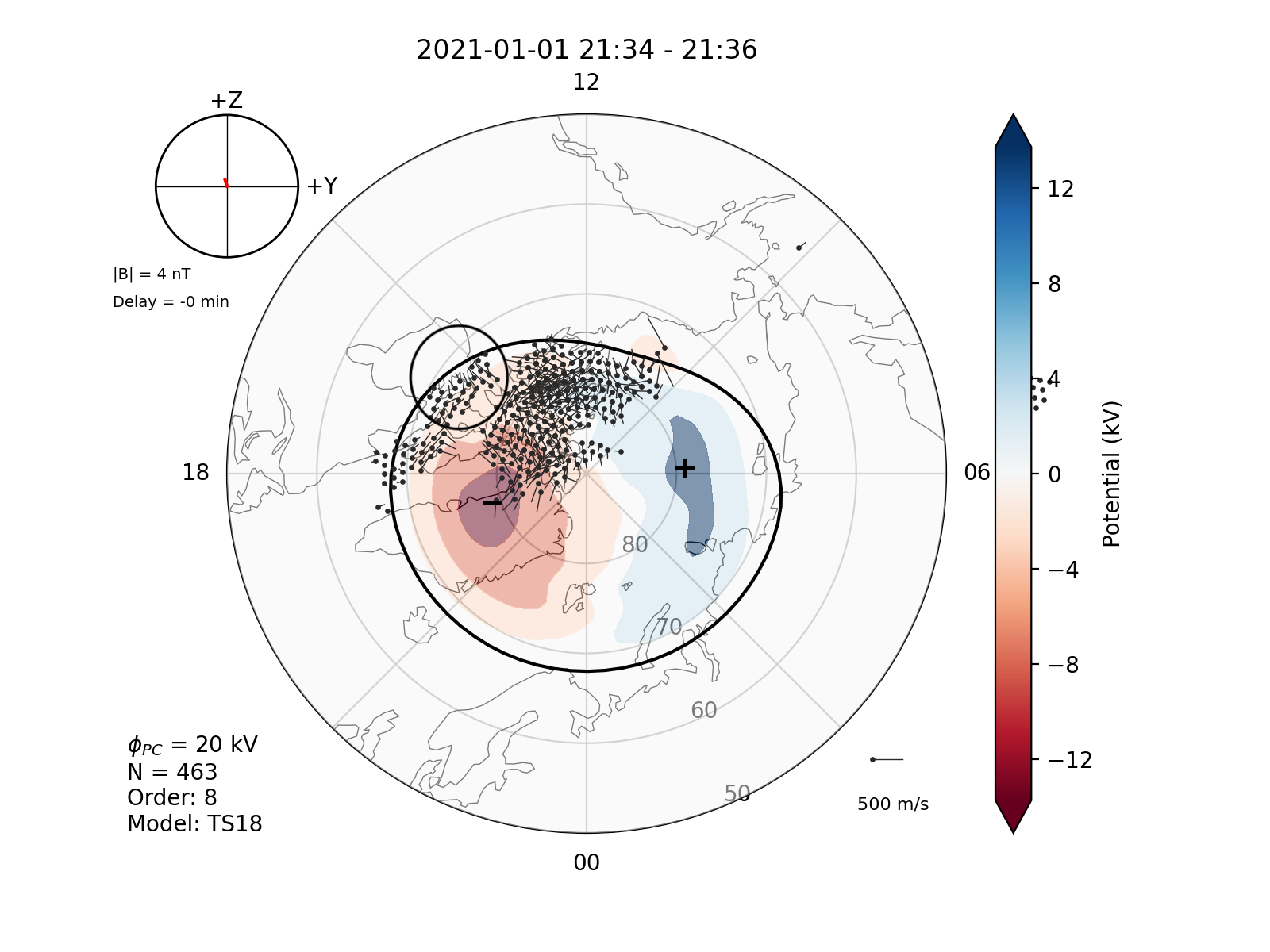
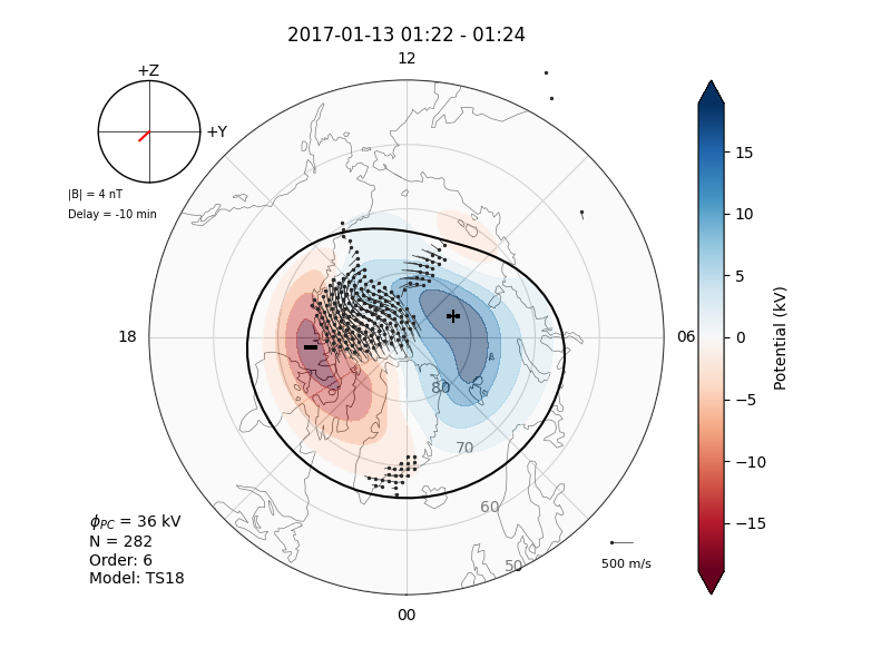
@carleyjmartin : We have an older IDL code (http://davit1.ece.vt.edu/doc/radar/rad_map_calc_true_vecs-code.html) written by Lasse Clausen that calculates True vectors. I compared the true vectors generated by pyDARN (Python version 3.9 and Matplotlib version 3.6.2) with the IDL estimates and noticed the results don't match. Not sure which one is correct but it might be worthwhile to double-check the code. I'm attaching the plots here, an example region with differences is between 15 and 17 MLT is circled. |
|
Hi Bharat, I've copied that version of code over to python to test, I'm not sure I have it 100% right yet, with both versions of code (my pydarn version and the python version of Lasse's IDL code) I'm still getting vectors that face outwards in the area circled. But there seems to be more differences in vector directions in general in the IDL converted code than with the new python code - I'm not sure what that is about but I'll keep having a go at it. The only thing I'm a little worried about is that the davit plot above in your comment looks very very similar to the fitted velocity plot, I'm wondering if the plotting function is plotting both the fitted and true as I can see that there are some places where there are more than one vector sock - which I would expect from plotting true velocities. Example of fitted velocity data for that date in pydarn (there will be some minor differences as we have different map files and mine is order 6): I've also converted over some old GO code that Dan has given me which he has used to produce true velocities in publications before.... all three versions give me something slightly different so it's possible that the exact definition of what we mean by true velocities and the exact calculation to do it in the community as a whole needs firming up. |
|
Ignore the above! I think I got it! There was some issues with vector components that I worked out. Example for the same date of newest version of true velocities (looks v.similar to yours now, with some minor differences due to map files and order): **Will push new version after commenting and tidying code up |
|
Hi @carleyjmartin, thanks for the quick turnaround on this. I think this newer version is much closer to the IDL version. However, there still are some minor differences. For example, between 16 & 18 MLT and near 80 MLAT, there are a few vectors that point predominantly equatorward in the latest pydarn code, whereas, the IDL version shows a poleward component. We might want to have another look at this before pushing the code. Let me know what you think. We don't necessarily have to assume the IDL code as the ground truth. |
This comment was marked as resolved.
This comment was marked as resolved.
|
In ubuntu, matplotlib 3.9.1 and numpy 1.26.4 I have fixed the problem. I have changed ".TRUE_VELOCITY" to ".RAW_VELOCITY" line 17: The plots are attached. |


From the appendix of Gareth's 2002 paper. “True” velocity vectors represent a combination of the average line-of-sight velocity measured at each grid cell with the component of the fit velocity vector which is perpendicular to the line-of-sight direction. [Figure A1c] presents a schematic representation of the true vector determination. The true vector (V_true) represents a velocity vector whose projection along the measured line-of-sight direction and the direction perpendicular to the line-of-sight direction match the measured line-of-sight velocity (V_los) and the perpendicular component of the fit vector (V_fit−perp), respectively. |
|
I have a few comments on this which might help (or not!). There is a comment earlier that on some of the true vec plots there are two vectors plotted at the same grid point. This is because there are often two LOS vectors in the same grid cell, which leads to 2 true vecs in that grid cell. I think to fully visually assess the true vec output, you need to plot the gridded LOS vectors as well as the fit and true. Then you can visually combine the LOS vectors with the perpendicular component of the fit vectors. So adding those plots for the examples above would be helpful for a visual assessment. I also looked at the calculated_true_velocities code and although not a python expert it did seem to match the original true vecs IDL code (pre Lasse/Ade) that Mike and Kile wrote. Although I had a question about the definitions of a_los and a_fit. Are these angles both zero to the north and positive eastward? I'm thinking that they are not both defined in the same way as in the k-vectors, kx for LOS is defined as -cos(a) and kx for FIT is defined as +cos(a). I can only think that this is because the angle definitions are different? Or is it because the LOS velocity is positive towards the radar, which might be opposite to the azimuth angle direction. Anyway, it might help to have this information in the comments in the code. (Also the descriptions of v_fit and a_fit are incorrect in the comments in the code). Anyway, if you add the gridded LOS plots alongside the FIT and TRUE ones, I'm happy to take a look. |
|
Thanks Gareth! Great idea! I'm trying to put together some plots to compare, but I've got 2 years of changes to update so I'm getting that out of the way first. At a quick glance it's really hard to see if the true vector looks reasonable compared to the LOS and fitted vectors, so I'm also trying to plot the perpendicular component of the fitted vector to make it clearer that it is a merge of the two of them. Also maps weren't designed to plot on top of each other so I'm not comparing directly, it's over three plots, attached below anyway, I'm not convinced it's right, looks a bit off. I also have a question about the a_los direction, it is read in purely from the map file (vector.kvect) and the RST documentation only says that it is 'Magnetic azimuth' in degrees so I don't really know where to find how it's officially defined, I think I've just been going about life assuming it is from N, +E. 


|
|
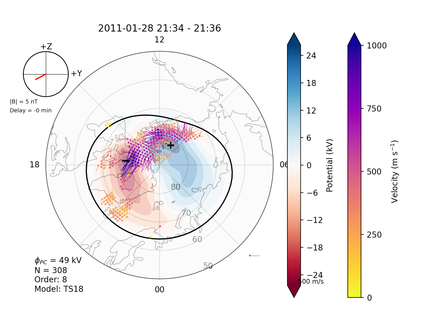
Better example: I'm pretty confident the clump around 18MLT 80 degrees is pointing in the wrong direction, and maybe the magnitude is too big? But then other clumps seem to make sense. I don't know why it looks like its clump dependent - maybe it is a negative issue with +/- LOS being weird. 


|
|
Yes, the true vectors in these examples look totally wrong. For the regions where the raw LOS and fitted vectors are close to being parallel the true vectors should also be close to this direction as the component of the fit vector that is perpendicular to the LOS vector is very small. But the true vectors appear to be going all over the place! As you say, being able to plot the perpendicular component of the fit vectors would probably be very helpful. As far as I know, the definition of the magnetic azimuth is as you state, zero to the north going positive to the east. I'll try and delve deeper and have another look at the code when I get some time. |
|
So, I have two questions about the code that don't make sense to me - although this might be python ignorance! First, as I mentioned above, the negative sign when setting the kx value for the LOS data. This seems odd as the vectors seem correctly aligned in the RAW plots you have added here, without this reversal in the kx value. So, I'd question this - this might be because things have changed with the definitions since Lasse's IDL code was written. Second, I am guessing that the sizes of the LOS and FIT arrays must be different, as there are often 2 LOS vectors at a single location? (Although not sure about this). How does the code identify that the two vectors being combined to create the TRUE vectors are at the same grid point? How do the lists for the two data sets line up? I think that these are possibly the source of the problems, so would be the area to concentrate on. |
|
Here's some follow up as I have been working on this on and off a little:
Code from potential_functions.pro in GO, no author stated in the file, but I believe it's Ade. Current Examples: LOS: FITTED: TRUE: I'm going to try and plot the fitted_perp vectors too. |


|
This example is the same as above but only using Rankin inlet data: LOS: FITTED: FITTED PERP TO LOS: You can see that it is perpendicular to the LOS velocity, but it's often in the wrong direction and definitely has the wrong magnitude... |


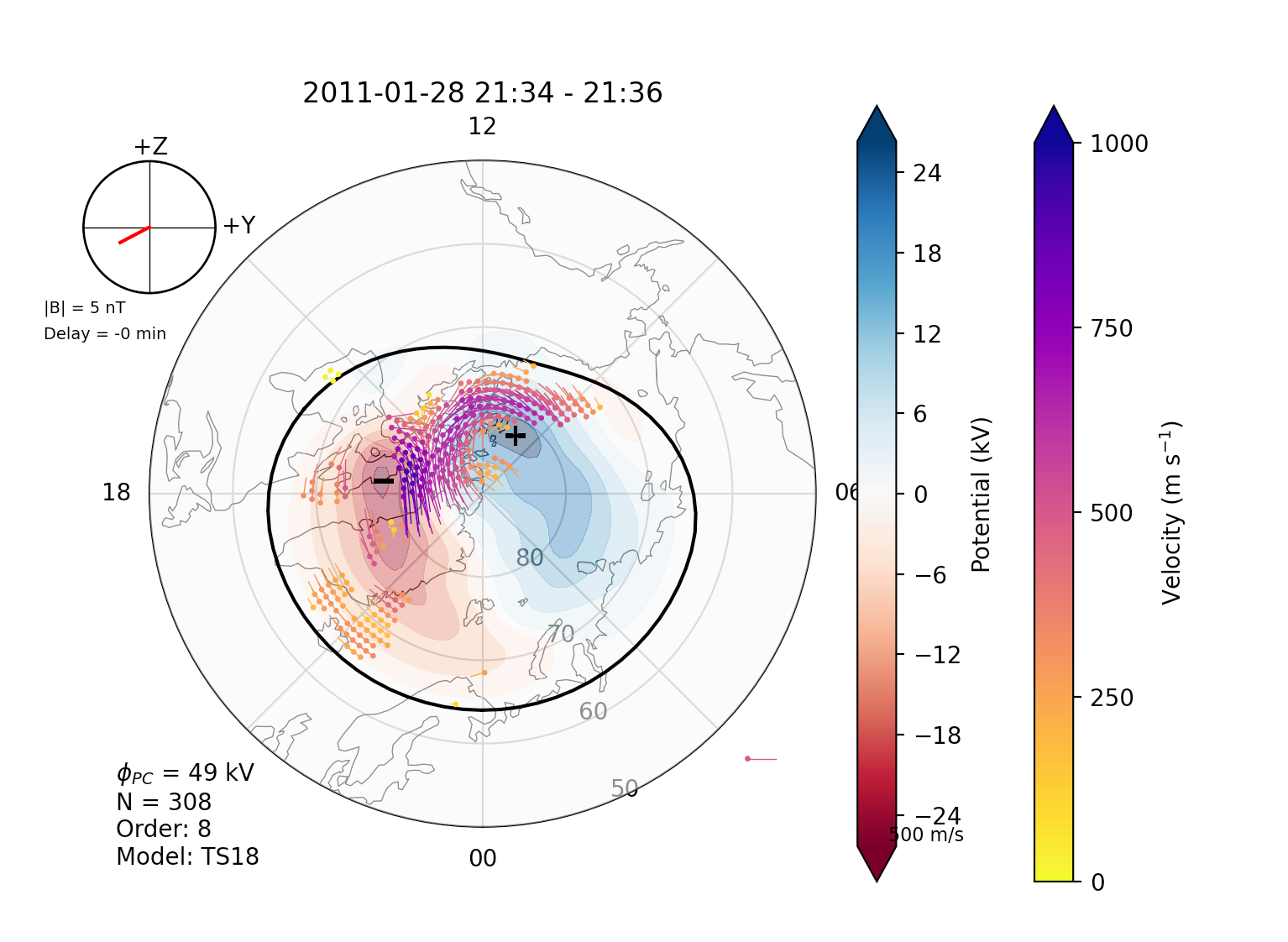
I think I've done it. It looks good. Turns out, I needed the -ve on the cos on the fitted components too. No idea why. LOS: FITTED: TRUE: 
|


|
Excellent news Carley. Well done. It seems that you have indeed fixed it. The vectors in the example that you've shown do definitely look correct. Interesting that it did seem to be a kx definition problem (if not exactly in the way that I'd thought) - having a different definition for kx for the FIT and LOS vectors did seem odd. It's very possible that something has changed since the old days. Then again it might have been something that was more deeply hidden in the IDL code. Have to say that the IDL code wasn't particularly clear in terms of what each command was doing!! Anyway, glad to know that you have it sorted. |
Scope
This PR adds the option to calculate and plot the true velocity vector. Where true velocity is the vector that is made from the LOS velocity and the perpendicular component of the fitted velocity to the LOS vector.
I need to validate the results from this with something that is published. If anyone has or knows of a paper with a time frame in this century and uses the newer model for fitting, but plots true vectors, please send it my way so I can compare and hopefully validate this calculation. I'm having trouble finding a suitable paper as a lot are using older models and 5 minute integrations, or the figures are just really unclear.
issue: to close #293
Approval
Number of approvals: 2 code review and testing (and possible validation to other data?)
Test
matplotlib version: 3.6.3
Note testers: please indicate what version of matplotlib you are using
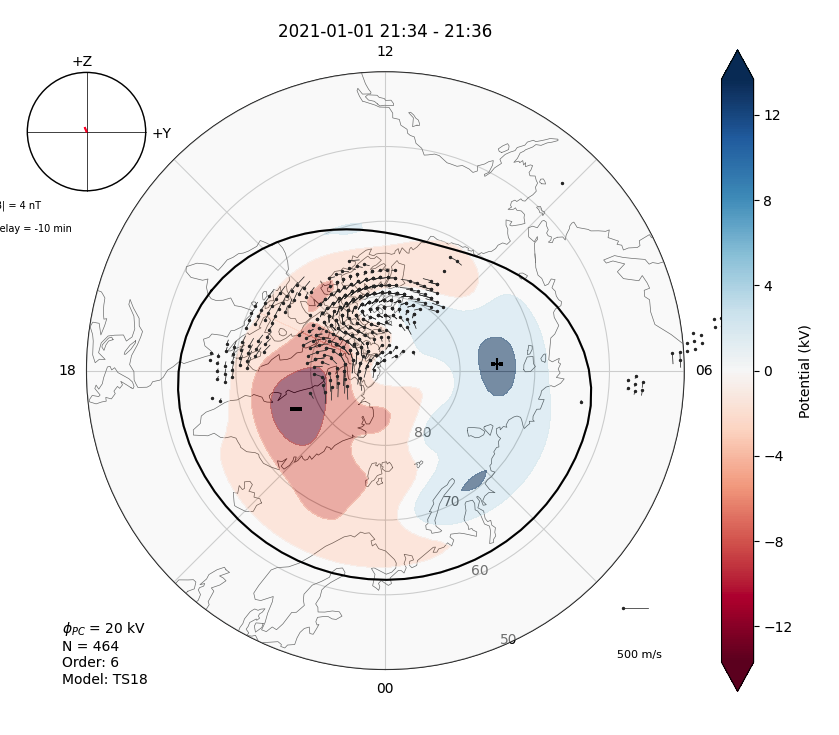
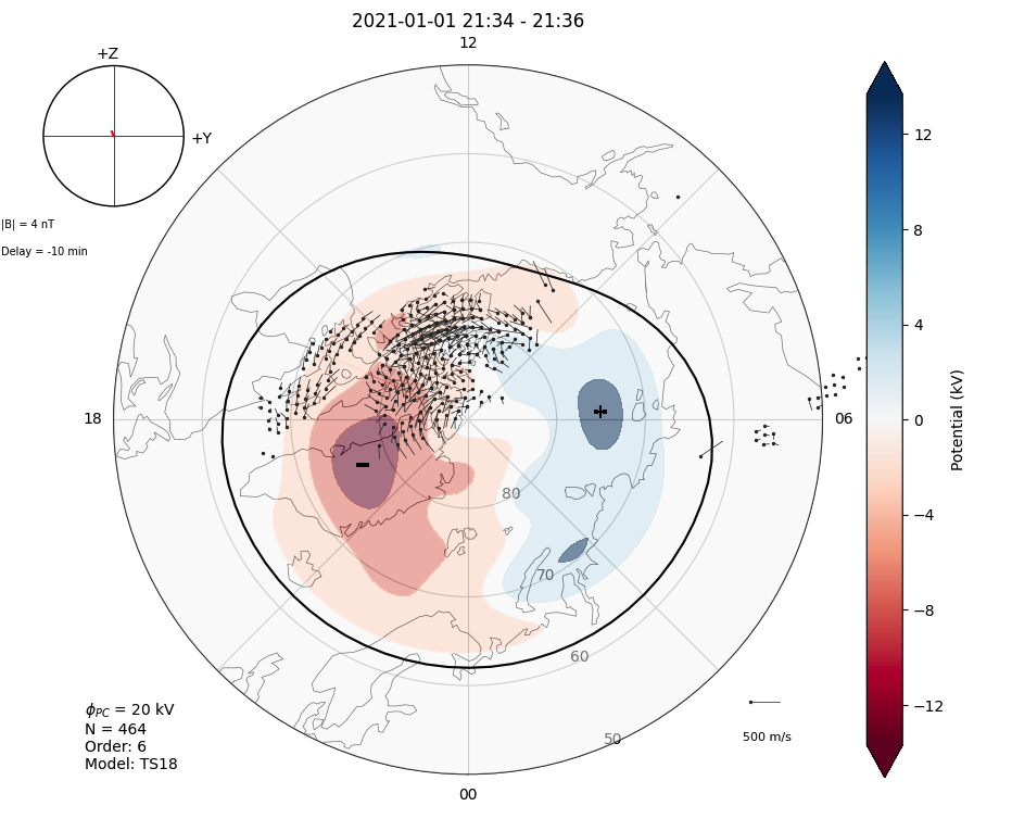
Code to compare true velocity vector and fitted velocity vectors.
Different time frame but you get the idea:

fitted
True
REPLACED IMAGES WITH UPDATED CODE:

LOS:
FITTED:

TRUE:
